AI画图原理与代码实现

论文介绍

Denoising Diffusion Probabilistic Models

论文作者为Jonathan Ho, 于2020年发布于NeurIPS, 与ICML, ICLR并称为机器学习三大顶会. 本论文是将扩散算法用于图像生成的开山之作.

前置知识

马尔可夫链

设某个系统在 $t$ 时刻的状态为 $X_t$ , 可以根据时间顺序得到一个序列 $P = \{X_t, X_{t-1}, \dots, X_0\}$ , 若前一时刻的状态只与上一时刻有关, 即

P(X_i | X_{i-1}, X_{i-2}, \cdots, X_0) = P(X_i | X_{i-1}) \tag{1-1}

则称其为马尔可夫链

重参数化

已知 $z \sim \mathcal{N}(z; \mu, \sigma^2 \bm{I})$ 表示 $z$ 是从均值为 $\mu$ , 方差为 $\sigma^2$ 的正态分布中采样得到的, 但是直接对其进行运算极为困难, 且不可导, 因此我们将随机性引入到变量 $\epsilon$ 上, 两者是可以相互转化的.

z = \mu + \sigma \cdot \epsilon, \epsilon \sim \mathcal{N}(0, \bm{I}) \tag{1-2}

贝叶斯公式

P(A | B) = \frac{P(B | A) \cdot P(A)}{P(B)} \tag{1-3}

在给定条件 $C$ 下

P(A | B, C) = \frac{P(B | A, C) \cdot P(A | C)}{P(B | C)} \tag{1-4}

证明如下:

\large \begin{array}{ll} & P(A|B,C) \\\\ =& \frac{P(B,C|A) \cdot P(A)}{P(B,C)} \\\\ =& \frac{P(B|A,C) \cdot P(C|A) \cdot P(A)}{P(B,C)} \\\\ =& \frac{P(B|A,C) \cdot P(A|C) \cdot P(C)}{P(B,C)} \\\\ =& \frac{P(B|A,C) \cdot P(A|C)}{P(B|C)} \end{array}

正态分布

若 $X \sim \mathcal{N}(\mu, \sigma^2)$ , 则

f(x) = \frac{1}{\sqrt{2 \pi}\sigma^2} \exp(-\frac{1}{2} \frac{(x-\mu)^2}{\sigma^2}) \tag{1-5}

可以发现前面的系数只与方差 $\sigma^2$ 有关, 因此在方差已经确定的情况下

f(x) \propto \exp(-\frac{1}{2} \frac{(x-\mu)^2}{\sigma^2}) \tag{1-6}

正向加噪

已有数据分布 $x_0 \sim q(x_0)$ , 向图中加入随机的高斯噪声, 得到 $x_1$ , 显然 $x_1$ 只与 $x_0$ 有关, 继续加入高斯噪声, 重复 $T$ 次, 得到 $x_T$ . 显然

q(x_1, \cdots, x_T | x_0) = \prod_{t=1}^T q(x_t | x_{t-1}) \tag{2-1}

由 $x_{t-1}$ 加入高斯噪声得到 $x_t$ 的过程可以表示为

q(x_t | x_{t-1}) = \mathcal{N}(x_t; \sqrt{1 - \beta_t} x_{t-1}, \beta_t \bm{I}) \tag{2-2}

其中 $\beta \in (0, 1)$ 是人为设定的超参数, 在计算开始前已经指定.

它还可以写为

x_t = \sqrt{\alpha_t}x_{t-1}+\sqrt{\beta_t}\epsilon_t, \epsilon_t \sim \mathcal{N}(0, \bm{I}), \alpha_t = 1 - \beta_t \tag{2-3}

使用该方法重复计算, 最终可以得到 $x_t$ , 但计算步骤过多, 算法性能极差, 因此我们需要想办法找到从 $x_0$ 与 $x_t$ 的快速算法

对 $x_{t-1}$ 进行迭代, 得到

\begin{array}{ll} x_t &= \sqrt{\alpha_t}x_{t-1}+\sqrt{\beta_t}\epsilon_t \\ &= \sqrt{\alpha_t}(\sqrt{\alpha_{t-1}}x_{t-2}+\sqrt{\beta_{t-1}}\epsilon_{t-1}) + \sqrt{\beta_t}\epsilon_t \\ &= \cdots \\ &= x_0 \prod_{i=1}^t \sqrt{\alpha_i} + \sqrt{\alpha_t \alpha_{t-1} \cdots \alpha_{2} \beta_1 } \epsilon_1 + \sqrt{\alpha_t \alpha_{t-1} \cdots \alpha_{3} \beta_2 } \epsilon_2 + \cdots + \sqrt{\alpha_t \beta_{t-1}} \epsilon_{t-1} + \sqrt{\beta_t} \epsilon_t \\ \end{array} \tag{2-4}

由于 $\epsilon_i \sim \mathcal{N}(0, \bm{I})$ , 因此我们可以将后面的全部项合并为一项.

例如:

\sqrt{\alpha_t \alpha_{t-1} \cdots \alpha_{2} \beta_1 } \epsilon_1 \sim \mathcal{N}(0, \alpha_t \alpha_{t-1} \cdots \alpha_{2} \beta_1 \bm{I}) \tag{2-5}

所以

\begin{array}{ll} & \mathcal{N}(0, \alpha_t \alpha_{t-1} \cdots \alpha_{2} \beta_1 \bm{I}) + \mathcal{N}(0, \alpha_t \alpha_{t-1} \cdots \alpha_{3} \beta_2 \bm{I}) + \cdots + \mathcal{N}(0, \alpha_t \beta_{t-1} \bm{I}) + \mathcal{N}(0, \beta_t \bm{I}) \\\\ =& \mathcal{N}\{0, \alpha_t \alpha_{t-1} \cdots \alpha_{2} (1-\alpha_1) \bm{I}\} + \mathcal{N}\{0, \alpha_t \alpha_{t-1} \cdots \alpha_{3} (1-\alpha_2) \bm{I}\} + \cdots + \mathcal{N}\{0, \alpha_t (1-\alpha_{t-1}) \bm{I}\} + \mathcal{N}\{0, (1-\alpha_t) \bm{I}\} \\\\ =& \mathcal{N}\{0, (\prod_{i=2}^t \alpha_i - \prod_{i=1}^t \alpha_i + \prod_{i=3}^t \alpha_i - \prod_{i=2}^t \alpha_i + \cdots + 1 - \alpha_t)\bm{I}\} \\\\ =& \mathcal{N}(0, 1 - \prod_{i=1}^t \alpha_i \bm{I}) \\\\ =& \mathcal{N}\{0, (1 - \bar{\alpha}) \bm{I}\}, \bar{\alpha} = \alpha_1 \alpha_2 \cdots \alpha_t \\\\ \end{array} \tag{2-6}

因此

p(x_t | x_0) = \sqrt{\bar{\alpha}} x_0 + \sqrt{1 - \bar{\alpha}} \epsilon = \mathcal{N}(x_t; \sqrt{\bar{\alpha}} x_0, (1-\bar{\alpha}) \bm{I}) , \epsilon \sim \mathcal{N}(0, \bm{I}) \tag{2-7}

也就是说, 只需要一步就可以由 $x_0$ 得到 $x_t$ . 这个结论将会在反向传播时用到.

由肉眼看来, 从 $x_0$ 到 $x_t$ 的过程, 就是图片被逐步加上高斯噪声, 不断杂乱化的过程. 此过程称为正向传播.

当步数 $t$ 足够大时, 以常识来看, 图片将会变成纯粹的高斯噪声图. 但在数学上, 仍需要严格证明. 由于 $\beta_t < 1$ 且 $t$ 趋向于无穷大, 因此

\lim_{n \rightarrow \infty} \bar{\alpha} = 0 \tag{2-8}

而通过上面的计算, 我们得知

p(x_t | x_0) = \mathcal{N}(x_t; \sqrt{\bar{\alpha}} x_0, (1-\bar{\alpha}) \bm{I}) \tag{2-9}

所以

\lim_{t \rightarrow \infty} q(x_t | x_0) = \mathcal{N}(0, \bm{I}), \lim_{t \rightarrow \infty} p(x_t) = \mathcal{N}(0, \bm{I}) \tag{2-10}

反向去噪

通过上面的过程, 我们有了逐步杂乱化的数据分布 $x_t$ , 计算机要做的是, 根据 $x_{t-1}$ , 倒推回 $x_t$ , 也就是从满是高斯噪声的图片, 反推回原图, 即求出 $q_\theta(x_{t-1} | x_t)$ . 此处的 $\theta$ 表示该参数是可学习的.

根据贝叶斯公式, 有

p(x_{t-1} | x_t) = \frac{p(x_t | x_{t-1}) \cdot p(x_{t-1})}{p(x_t)} \tag{3-1}

但 $p(x_{t-1})$ 和 $p(x_t)$ 是未知的, 我们可以给定条件 $x_0$ , 则原等式变为

p(x_{t-1} | x_t, x_0) = \frac{p(x_t | x_{t-1}, x_0) \cdot p(x_{t-1} | x_0)}{p(x_t | x_0)} \tag{3-2}

根据马尔可夫链的性质, 我们知道下一状态只与上一状态有关, 所以 $p(x_t | x_{t-1}, x_0) = p(x_t | x_{t-1})$ , 因此

p(x_{t-1} | x_t, x_0) = \frac{p(x_t | x_{t-1}) \cdot p(x_{t-1} | x_0)}{p(x_t | x_0)} \tag{3-3}

根据公式 $(2-1)$ 和 $(2-2)$ , 我们可以写出以下三个表达式:

\large \begin{array}{ll} 1. p(x_t | x_{t-1}) &\sim \mathcal{N}(\sqrt{\alpha_t}x_{t-1}, (1 - \alpha_t)\bm{I}) \\ 2. p(x_{t-1} | x_0) &\sim \mathcal{N}(\sqrt{\bar{\alpha}_{t-1}}x_0, (1 - \bar{\alpha}_{t-1})\bm{I}) \\ 3. p(x_t | x_0) &\sim \mathcal{N}(\sqrt{\bar{\alpha}_t}x_0, (1 - \bar{\alpha}_t)\bm{I}) \end{array} \tag{3-4}

注意第一个不是 $\bar{\alpha}_t$ , 而是 $\alpha_t$ , 因为 $\bar{\alpha}_t = \alpha_1 \alpha_2 \cdots \alpha_t$ , 而从 $x_{t-1}$ 扩散到 $x_t$ 只需要一步

可以发现, 以上三项全部都是正态分布, 其中方差均为超参数, 是人为指定的常数, 即正态分布的系数也是预先确定的常数, 所以我们不关心系数具体是什么, 因而有

\Large \begin{array}{ll} & p(x_{t-1} | x_t, x_0) \\\\ \propto & \exp{\left\{ -\frac12 \left[ \frac{(x_t - \sqrt{\alpha_t}x_{t-1})^2}{\beta_t} + \frac{(x_{t-1} - \sqrt{\bar{\alpha}_{t-1}}x_0)^2}{1-\bar{\alpha}_{t-1}} - \frac{(x_t - \sqrt{\bar{\alpha}_t}x_0)^2}{1-\bar{\alpha}_t} \right]\right\}} \\\\ = & \exp{\left[ -\frac12 \left( \frac{x_t^2}{\beta_t} - \frac{2\sqrt{\alpha_t}x_t x_{t-1}}{\beta_t} + \frac{\alpha_t x_{t-1}^2}{\beta_t} + \frac{x_{t-1}^2}{1-\bar{\alpha}_{t-1}}\right. \right.} - \frac{2\sqrt{\bar{\alpha}_{t-1}}x_0 x_{t-1}}{1-\bar{\alpha}_{t-1}} \\\\ & \left.\left. + \frac{\bar{\alpha}_{t-1} x_0^2}{1-\bar{\alpha}_{t-1}} - \frac{x_t^2}{1-\bar{\alpha}_t} + \frac{2\sqrt{\bar{\alpha}_t}x_0 x_t}{1-\bar{\alpha}_t} - \frac{\bar{\alpha}_t x_0^2}{1-\bar{\alpha}_t} \right)\right] \\\\ =& \exp{\left\{ -\frac12 \left[ \left(\frac{\alpha_t}{\beta_t} + \frac1{1-\bar{\alpha}_{t-1}}\right)x_{t-1}^2 - \left(\frac{2\sqrt{\alpha_t}}{\beta_t}x_t + \frac{2\sqrt{\bar{\alpha}_{t-1}}}{1-\bar{\alpha}_{t-1}}x_0\right)x_{t-1} + C(x_0, x_t) \right]\right\}} \end{array} \tag{3-5}

其中 $C(x_0, x_t)$ 是关于 $x_0, x_t$ 的常数项, 仔细观察下列两个式子

我们知道正态分布化开后是

\exp\left\{-\frac{(x-\mu)^2}{2\sigma^2}\right\} = \exp\left\{-\frac12 \left( \frac1{\sigma^2}x^2 - \frac{2\mu}{\sigma^2}x + \frac{\mu^2}{\sigma^2} \right) \right\} \tag{3-6}

与上面得到的结果仔细比对

\large \begin{array}{ll} \exp\left\{ -\frac12 \left[ \left(\frac{\alpha_t}{\beta_t} + \frac1{1-\bar{\alpha}_{t-1}}\right) x_{t-1}^2 - \left(\frac{2\sqrt{\alpha_t}}{\beta_t}x_t + \frac{2\sqrt{\bar{\alpha}_{t-1}}}{1-\bar{\alpha}_{t-1}}x_0\right)x_{t-1} + C(x_0, x_t) \right]\right\} \\\\ \exp\left\{-\frac12 \left[ \frac1{\sigma^2} x^2 - \frac{2\mu}{\sigma^2}x + \frac{\mu^2}{\sigma^2} \right] \right\} \end{array} \tag{3-7}

可以发现上下各项都可以一一对应, 即 $p(x_{t-1} | x_t, x_0)$ 的结果又是一个正态分布, 我们可以轻易看出这个新的正态分布的参数

\Large \begin{array}{ll} \tilde\sigma^2 &= \frac{\beta_t (1-\bar{\alpha}_{t-1})}{\alpha_t - \alpha_t \bar{\alpha}_{t-1} + \beta_t} = \frac{\beta_t (1-\bar{\alpha}_{t-1})}{1-\bar{\alpha}_t} \\\\ \tilde\mu &= \frac{\sqrt{\alpha_t}(1-\bar{\alpha}_{t-1})}{1-\bar{\alpha}_t}x_t + \frac{\beta_t \sqrt{\bar{\alpha}_{t-1}}}{1-\bar{\alpha}_t}x_0 \end{array} \tag{3-8}

根据公式 $(2-7)$ , 我们有

x_0 = \frac{1}{\sqrt{\bar{\alpha}_t}}\left( x_t - \sqrt{1-\bar{\alpha}_t}\epsilon_t \right) \tag{3-9}

代入公式 $(3-8)$ , 得到

\Large \begin{array}{ll} \tilde\mu &= \left[ \frac{\sqrt{\alpha_t}(1-\bar{\alpha}_{t-1})}{1-\bar{\alpha}_t} + \frac{\beta_t \sqrt{\bar{\alpha}_{t-1}}}{(1-\bar{\alpha}_t) \sqrt{\bar{\alpha}_t}} \right] x_t - \frac{\beta_t \sqrt{\bar{\alpha}_{t-1}}\sqrt{1-\bar{\alpha}_t}}{(1-\bar{\alpha}_t) \sqrt{\bar{\alpha}_t}} \epsilon_t \\\\ &= \frac{\sqrt{\alpha_t} \cdot \sqrt{\bar{\alpha}_t}(1-\bar{\alpha}_{t-1})+\beta_t \sqrt{\bar{\alpha}_{t-1}}}{(1-\bar{\alpha}_t)\sqrt{\bar{\alpha}_t}} x_t - \frac{\beta_t \sqrt{1-\bar{\alpha}_t}}{(1-\bar{\alpha}_t) \cdot \sqrt{\alpha_t}} \epsilon_t \\\\ &= \frac{\alpha_t \cdot \sqrt{\bar{\alpha}_{t-1}} (1-\bar{\alpha}_{t-1}) + \beta_t \sqrt{\bar{\alpha}_{t-1}}}{(1-\bar{\alpha}_t) \sqrt{\bar{\alpha}_t}}x_t - \frac{\beta_t}{\sqrt{1-\bar{\alpha}_t} \cdot \sqrt{\alpha_t}} \epsilon_t \\\\ &= \frac{\sqrt{\bar{\alpha}_{t-1}}(\alpha_t - \bar{\alpha}_t + \beta_t)}{(1-\bar{\alpha}_t)\sqrt{\bar{\alpha}_t}} x_t - \frac{\beta_t}{\sqrt{1-\bar{\alpha}_t} \cdot \sqrt{\alpha_t}} \epsilon_t \\\\ &= \frac{1}{\sqrt{\alpha}_t}\left( x_t - \frac{\beta_t}{\sqrt{1-\bar{\alpha}_t}}\epsilon_t \right) \end{array} \tag{3-10}

最后我们就可以用 $x_t$ 反向求出 $x_{t-1}$ :

\Large x_{t-1} = \tilde \mu + \tilde \sigma \epsilon = \frac{1}{\sqrt{\alpha}_t}\left( x_t - \frac{\beta_t}{\sqrt{1-\bar{\alpha}_t}}\epsilon_t \right) + \sqrt{\frac{\beta_t (1-\bar{\alpha}_{t-1})}{1-\bar{\alpha}_t}} \epsilon \tag{3-11}

模型代码

残差网络

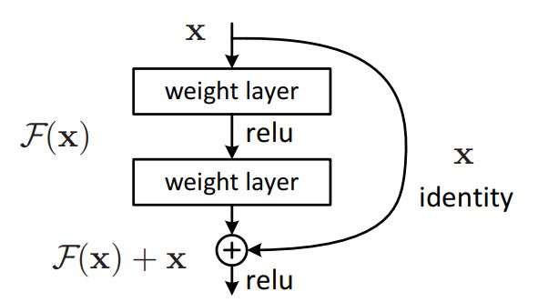
多层神经网络会出现梯度消失和梯度爆炸现象, 其准确度甚至无法达到层数更少的神经网络. 实际上, 由数据处理不等式(DPI)可得, 信息在多层网络直接传播的过程中, 下一层所包含的信息总是小于上一层. 论文Deep Residual Learning for Image Recognition提出, 使用 $Y = X + F(X, W)$ 代替 $Y = F(X)$ , 可以让原始数据直接传递到更深层, 从而让深层网络包含的信息总是大于浅层网络.

代码如下:

class ResNet(nn.Module):
    def __init__(self,
                 channel_input: int,
                 channel_output: int,
                 channel_time: int,
                 device: str = 'cpu'):
        """
        :param channel_input: 输入通道数
        :param channel_output: 输出通道数
        :param channel_time: 时间通道数
        """
        super().__init__()
        self.conv1 = nn.Sequential(
            nn.GroupNorm(32, channel_input, device=device),
            nn.SiLU(),
            nn.Conv2d(channel_input, channel_output, kernel_size=3, padding=1)
        )

        self.time_embedding = nn.Sequential(
            nn.SiLU(),
            nn.Linear(channel_time, channel_output)
        )

        self.conv2 = nn.Sequential(
            nn.GroupNorm(32, channel_output, device=device),
            nn.SiLU(),
            nn.Conv2d(channel_output, channel_output, kernel_size=3, padding=1)
        )

        if channel_input == channel_output:
            self.shortcut = nn.Identity()
        else:
            self.shortcut = nn.Conv2d(channel_input, channel_output, kernel_size=1)

        self.to(device)

    def forward(self, x: torch.Tensor, t: torch.Tensor) -> torch.Tensor:
        """
        :param x: [batch_size, channel_input, h, w]
        :param t: [batch_size, channel_time]
        :return: [batch_size, channel_output, h, w]
        """
        result = self.conv1(x)
        result += self.time_embedding(t)[:, :, None, None]
        result = self.conv2(result)
        return result + self.shortcut(x)

注意力机制

一般的注意力机制公式如下:

out = softmax(\frac{QK^\top}{\sqrt{d_k}})V^\top

其中 $Q, K, V$ 都是通过卷积得来的

现已有原图 $X \in \mathbb{R}^{C \times H \times W}$ , 其三个维度分别是通道, 高, 宽. 将高与宽合并为一维, 得到 $X' \in \mathbb{R}^{C \times (H \times W)}$

通过卷积的方法, 可以将其转化为三个矩阵

Q, K \in \mathbb{R}^{C / r \times (H \times W)} \\ V \in \mathbb{R}^{C \times (H \times W)}

由于 channel 通道在第一维, 所以整个公式也要转置一下

out = V \left[softmax \left( \frac{Q^\top K}{\sqrt{d_k}} \right) \right]^\top \in \mathbb{R}^{C \times (H \times W)}

其中 $d_k$ 是通道数 $C$

class AttentionBlock(nn.Module):
    def __init__(self, in_channels, device='cpu'):
        super().__init__()

        self.query_conv = nn.Conv2d(in_channels, in_channels // 8, kernel_size=1, bias=False)
        self.key_conv = nn.Conv2d(in_channels, in_channels // 8, kernel_size=1, bias=False)
        self.value_conv = nn.Conv2d(in_channels, in_channels, kernel_size=1, bias=False)

        self.to(device)

    def forward(self, x, t):
        batch_size, channels, height, width = x.shape

        query = self.query_conv(x).view(batch_size, -1, height * width).permute(0, 2, 1)
        key = self.key_conv(x).view(batch_size, -1, height * width)
        value = self.value_conv(x).view(batch_size, -1, height * width)

        attention = torch.bmm(query, key) / math.sqrt(key.shape[1])
        attention = F.softmax(attention, dim=-1)

        out = torch.bmm(value, attention.permute(0, 2, 1))
        out = out.view(batch_size, channels, height, width)

        out = out + x
        return out

UNet

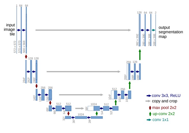
UNet模型不需要过多数学知识, 这里直接给出代码. 但有一点需要注意, 有些模型只有一个输入, 为了便于编码, 全部改为了两个输入, 第二个输入是 timestep, 在部分模型中仅用于占位.

class DownSample(nn.Module):
    def __init__(self, channels: int, device: str = 'cpu'):
        super().__init__()
        self.op = nn.Conv2d(channels, channels, kernel_size=3, stride=2, padding=1)
        self.to(device)

    def forward(self, x: torch.Tensor, t: torch.Tensor) -> torch.Tensor:
        """
        返回下采样后的图
        :param x: [channel, h, w]
        :param t: 占位
        :return: [channel, h, w]
        """
        return self.op(x)


class UpSample(nn.Module):
    def __init__(self, channels: int, device: str = 'cpu'):
        super().__init__()
        self.op = nn.Conv2d(channels, channels, kernel_size=3, padding=1)
        self.to(device)

    def forward(self, x: torch.Tensor, t: torch.Tensor) -> torch.Tensor:
        """
        返回上采样后的图
        :param x: [channel, h, w]
        :param t: 占位
        :return:
        """
        x = F.interpolate(x, scale_factor=2, mode="nearest")
        x = self.op(x)
        return x


class ModuleList(nn.Module):
    def __init__(self, *args):
        super().__init__()
        self.module_list = []
        for idx, module in enumerate(args):
            self.module_list.append(module)

    def forward(self, x: torch.Tensor, t: torch.Tensor) -> torch.Tensor:
        for module in self.module_list:
            x = module(x, t)
        return x


class ModuleAdapter(nn.Module):
    def __init__(self, module):
        super().__init__()
        self.module = module

    def forward(self, x: torch.Tensor, t: torch.Tensor):
        return self.module(x)


class UNetModel(nn.Module):
    def __init__(self,
                 channel_input: int = 3,
                 channel_output: int = 3,
                 channel_model: int = 128,
                 channel_time: int = 512,
                 device: str = 'cpu'
                 ):
        super().__init__()
        self.channel_input = channel_input
        self.channel_output = channel_output
        self.channel_model = channel_model

        self.time_embedding = nn.Sequential(
            nn.Linear(channel_model, channel_time),
            nn.SiLU(),
            nn.Linear(channel_time, channel_time)
        )

        self.down_blocks = nn.ModuleList([
            ModuleAdapter(nn.Conv2d(3, 128, kernel_size=3, stride=1, padding=1)),
            ResNet(128, 128, channel_time, device=device),
            ResNet(128, 128, channel_time, device=device),
            DownSample(128, device=device),
            ModuleList(
                ResNet(128, 256, channel_time, device=device),
                AttentionBlock(256, device=device),
            ),
            ModuleList(
                ResNet(256, 256, channel_time, device=device),
                AttentionBlock(256, device=device),
            ),
            DownSample(256, device=device),
            ResNet(256, 256, channel_time, device=device),
            ResNet(256, 256, channel_time, device=device),
            DownSample(256, device=device),
            ResNet(256, 256, channel_time, device=device),
            ResNet(256, 256, channel_time, device=device),
        ])

        self.up_blocks = nn.ModuleList([
            ResNet(512, 256, channel_time, device=device),
            ResNet(512, 256, channel_time, device=device),
            ModuleList(
                ResNet(512, 256, channel_time, device=device),
                UpSample(256, device=device),
            ),
            ResNet(512, 256, channel_time, device=device),
            ResNet(512, 256, channel_time, device=device),
            ModuleList(
                ResNet(512, 256, channel_time, device=device),
                UpSample(256, device=device),
            ),
            ModuleList(
                ResNet(512, 256, channel_time, device=device),
                AttentionBlock(256, device=device),
            ),
            ModuleList(
                ResNet(512, 256, channel_time, device=device),
                AttentionBlock(256, device=device),
            ),
            ModuleList(
                ResNet(384, 256, channel_time, device=device),
                AttentionBlock(256, device=device),
                UpSample(256, device=device),
            ),
            ResNet(384, 128, channel_time, device=device),
            ResNet(256, 128, channel_time, device=device),
            ResNet(256, 128, channel_time, device=device),
        ])

        self.middle = ModuleList(
            ResNet(256, 256, channel_time, device=device),
            AttentionBlock(256, device=device),
            ResNet(256, 256, channel_time, device=device),
        )

        self.out = nn.Sequential(
            nn.GroupNorm(32, 128, device=device),
            nn.SiLU(),
            nn.Conv2d(128, 3, kernel_size=3, padding=1)
        )

        self.to(device)

    def forward(self, x: torch.Tensor, t: torch.Tensor) -> torch.Tensor:
        """
        :param x:
        :param t:
        :return:
        """
        emb = self.time_embedding(timestep_embedding(t, self.channel_model))
        hs = []
        h = x
        for module in self.down_blocks:
            h = module(h, emb)
            hs.append(h)
        h = self.middle(h, emb)
        for module in self.up_blocks:
            temp = torch.cat([h, hs.pop()], dim=1)
            h = module(temp, emb)
        return self.out(h)

完整代码

目前这些代码仍有部分问题, 且训练图尺寸与生成图尺寸不同时还会出现图片畸形. 但对初学者来说已足够了解模型思想. 在阅读 DDPM 的构造函数与生成函数时, 建议与上面的公式进行对照, 以方便理解代码含义.

将以下文件放入同一个文件夹中. 先用 Data.py 生成数据集文件, 然后修改 config.yml 里的配置, 最后运行 train.py 即可.

最后, 训练时建议用同一类图片或同一个数据集进行训练, 可以先将学习率设置为 1e-3 训练 50 轮, 再改为 2e-4 训练 200 轮, 再改为 2e-5, 2e-6 分别训练 500, 1000 轮. 每次训练好先看一下效果再决定是否继续训练. 如果训练轮次太高可能会出现 loss 上升, 效果反而变差, 所以继续训练时先备份一下上一个模型.

训练图尺寸和 batch_size 根据你的显存调整, 一般 6G 以内建议用 32×32, 12~24G 用 64×64, 不建议 128×128 或更高, 显存会达到恐怖的 78G, 需要专业计算卡, 除非改用很小的 batch_size

下面是我提供的训练集和模型, 对应的尺寸为 32×32, 在 generate.py 里面修改.未来可能会上传其他尺寸的模型, 注意看一下文件名改一下生成尺寸.

百度网盘(提取码:6666)

https://pan.baidu.com/s/1ZKPUfqW8nVitedOiadu-MA?pwd=6666

私人云盘

https://pan.dearxuan.com/s/jRfM

效果如下

Data.py

import glob
import os.path as path

import numpy as np
import torch
from PIL import Image
from torchvision import transforms


def save_to_file(size: int = 64,
                 img_dir: str = './images/',
                 file: str = './images/img.pth'):
    data_transforms = [
        transforms.Resize((size, size)),  # 缩放
        transforms.ToTensor(),  # 将原本像素范围 [0, 255] 的图像转化为范围 [0, 1] 的张量
        transforms.Lambda(lambda t: (t * 2) - 1)  # 调整范围至 [-1, 1], 或者用 transform.Normalize()
    ]
    data_transform = transforms.Compose(data_transforms)
    files = sorted(glob.glob(path.join(img_dir, '*')))
    images = [data_transform(Image.open(file)) for file in files]
    images = torch.tensor(np.array(images), dtype=torch.float32)
    torch.save(images, file)


if __name__ == '__main__':
    save_to_file(size=64, img_dir='./images/256/', file='./images/girls_64.pth')

DDPModel.py

import math

import numpy as np
import torch
import torch.nn as nn
import torch.nn.functional as F
from tqdm import tqdm


def timestep_embedding(timesteps, dim, max_period=10000):
    """
    timestep 正弦嵌入
    :param timesteps: a 1-D Tensor of N indices, one per batch element.
                      These may be fractional.
    :param dim: the dimension of the output.
    :param max_period: controls the minimum frequency of the embeddings.
    :return: an [N x dim] Tensor of positional embeddings.
    """
    half = dim // 2
    freqs = torch.exp(
        -math.log(max_period) * torch.arange(start=0, end=half, dtype=torch.float32) / half
    ).to(device=timesteps.device)
    args = timesteps[:, None].float() * freqs[None]
    embedding = torch.cat([torch.cos(args), torch.sin(args)], dim=-1)
    if dim % 2:
        embedding = torch.cat([embedding, torch.zeros_like(embedding[:, :1])], dim=-1)
    return embedding


class ResNet(nn.Module):
    def __init__(self,
                 channel_input: int,
                 channel_output: int,
                 channel_time: int,
                 device: str = 'cpu'):
        """
        :param channel_input: 输入通道数
        :param channel_output: 输出通道数
        :param channel_time: 时间通道数
        """
        super().__init__()
        self.conv1 = nn.Sequential(
            nn.GroupNorm(32, channel_input, device=device),
            nn.SiLU(),
            nn.Conv2d(channel_input, channel_output, kernel_size=3, padding=1)
        )

        self.time_embedding = nn.Sequential(
            nn.SiLU(),
            nn.Linear(channel_time, channel_output)
        )

        self.conv2 = nn.Sequential(
            nn.GroupNorm(32, channel_output, device=device),
            nn.SiLU(),
            nn.Conv2d(channel_output, channel_output, kernel_size=3, padding=1)
        )

        if channel_input == channel_output:
            self.shortcut = nn.Identity()
        else:
            self.shortcut = nn.Conv2d(channel_input, channel_output, kernel_size=1)

        self.to(device)

    def forward(self, x: torch.Tensor, t: torch.Tensor) -> torch.Tensor:
        """
        :param x: [batch_size, channel_input, h, w]
        :param t: [batch_size, channel_time]
        :return: [batch_size, channel_output, h, w]
        """
        result = self.conv1(x)
        result += self.time_embedding(t)[:, :, None, None]
        result = self.conv2(result)
        return result + self.shortcut(x)


class AttentionBlock(nn.Module):
    def __init__(self, in_channels, device='cpu'):
        super().__init__()

        self.query_conv = nn.Conv2d(in_channels, in_channels // 8, kernel_size=1, bias=False)
        self.key_conv = nn.Conv2d(in_channels, in_channels // 8, kernel_size=1, bias=False)
        self.value_conv = nn.Conv2d(in_channels, in_channels, kernel_size=1, bias=False)

        self.to(device)

    def forward(self, x, t):
        batch_size, channels, height, width = x.shape

        query = self.query_conv(x).view(batch_size, -1, height * width).permute(0, 2, 1)
        key = self.key_conv(x).view(batch_size, -1, height * width)
        value = self.value_conv(x).view(batch_size, -1, height * width)

        attention = torch.bmm(query, key) / math.sqrt(key.shape[1])
        attention = F.softmax(attention, dim=-1)

        out = torch.bmm(value, attention.permute(0, 2, 1))
        out = out.view(batch_size, channels, height, width)

        out = out + x
        return out


class DownSample(nn.Module):
    def __init__(self, channels: int, device: str = 'cpu'):
        super().__init__()
        self.op = nn.Conv2d(channels, channels, kernel_size=3, stride=2, padding=1)
        self.to(device)

    def forward(self, x: torch.Tensor, t: torch.Tensor) -> torch.Tensor:
        """
        返回下采样后的图
        :param x: [channel, h, w]
        :param t: 占位
        :return: [channel, h, w]
        """
        return self.op(x)


class UpSample(nn.Module):
    def __init__(self, channels: int, device: str = 'cpu'):
        super().__init__()
        self.op = nn.Conv2d(channels, channels, kernel_size=3, padding=1)
        self.to(device)

    def forward(self, x: torch.Tensor, t: torch.Tensor) -> torch.Tensor:
        """
        返回上采样后的图
        :param x: [channel, h, w]
        :param t: 占位
        :return:
        """
        x = F.interpolate(x, scale_factor=2, mode="nearest")
        x = self.op(x)
        return x


class ModuleList(nn.Module):
    def __init__(self, *args):
        super().__init__()
        self.module_list = []
        for idx, module in enumerate(args):
            self.module_list.append(module)

    def forward(self, x: torch.Tensor, t: torch.Tensor) -> torch.Tensor:
        for module in self.module_list:
            x = module(x, t)
        return x


class ModuleAdapter(nn.Module):
    def __init__(self, module):
        super().__init__()
        self.module = module

    def forward(self, x: torch.Tensor, t: torch.Tensor):
        return self.module(x)


class UNetModel(nn.Module):
    def __init__(self,
                 channel_input: int = 3,
                 channel_output: int = 3,
                 channel_model: int = 128,
                 channel_time: int = 512,
                 device: str = 'cpu'
                 ):
        super().__init__()
        self.channel_input = channel_input
        self.channel_output = channel_output
        self.channel_model = channel_model

        self.time_embedding = nn.Sequential(
            nn.Linear(channel_model, channel_time),
            nn.SiLU(),
            nn.Linear(channel_time, channel_time)
        )

        self.down_blocks = nn.ModuleList([
            ModuleAdapter(nn.Conv2d(3, 128, kernel_size=3, stride=1, padding=1)),
            ResNet(128, 128, channel_time, device=device),
            ResNet(128, 128, channel_time, device=device),
            DownSample(128, device=device),
            ModuleList(
                ResNet(128, 256, channel_time, device=device),
                AttentionBlock(256, device=device),
            ),
            ModuleList(
                ResNet(256, 256, channel_time, device=device),
                AttentionBlock(256, device=device),
            ),
            DownSample(256, device=device),
            ResNet(256, 256, channel_time, device=device),
            ResNet(256, 256, channel_time, device=device),
            DownSample(256, device=device),
            ResNet(256, 256, channel_time, device=device),
            ResNet(256, 256, channel_time, device=device),
        ])

        self.up_blocks = nn.ModuleList([
            ResNet(512, 256, channel_time, device=device),
            ResNet(512, 256, channel_time, device=device),
            ModuleList(
                ResNet(512, 256, channel_time, device=device),
                UpSample(256, device=device),
            ),
            ResNet(512, 256, channel_time, device=device),
            ResNet(512, 256, channel_time, device=device),
            ModuleList(
                ResNet(512, 256, channel_time, device=device),
                UpSample(256, device=device),
            ),
            ModuleList(
                ResNet(512, 256, channel_time, device=device),
                AttentionBlock(256, device=device),
            ),
            ModuleList(
                ResNet(512, 256, channel_time, device=device),
                AttentionBlock(256, device=device),
            ),
            ModuleList(
                ResNet(384, 256, channel_time, device=device),
                AttentionBlock(256, device=device),
                UpSample(256, device=device),
            ),
            ResNet(384, 128, channel_time, device=device),
            ResNet(256, 128, channel_time, device=device),
            ResNet(256, 128, channel_time, device=device),
        ])

        self.middle = ModuleList(
            ResNet(256, 256, channel_time, device=device),
            AttentionBlock(256, device=device),
            ResNet(256, 256, channel_time, device=device),
        )

        self.out = nn.Sequential(
            nn.GroupNorm(32, 128, device=device),
            nn.SiLU(),
            nn.Conv2d(128, 3, kernel_size=3, padding=1)
        )

        self.to(device)

    def forward(self, x: torch.Tensor, t: torch.Tensor) -> torch.Tensor:
        """
        :param x:
        :param t:
        :return:
        """
        emb = self.time_embedding(timestep_embedding(t, self.channel_model))
        hs = []
        h = x
        for module in self.down_blocks:
            h = module(h, emb)
            hs.append(h)
        h = self.middle(h, emb)
        for module in self.up_blocks:
            temp = torch.cat([h, hs.pop()], dim=1)
            h = module(temp, emb)
        return self.out(h)


class DDPM(nn.Module):
    def __init__(self,
                 timestep: int = 1000,
                 beta_start: int = 0.0001,
                 beta_end: int = 0.02,
                 device: str = 'cpu'):
        """
        :param timestep: 步数, 默认为 1000
        :param beta_start: beta起始值
        :param beta_end: beta结束值
        :param tensor_range: 数据集转为tensor的范围: [-range, range]
        """
        super().__init__()
        self.timestep = timestep
        self.beta_start = beta_start
        self.beta_end = beta_end
        self.device = device
        self.unet = UNetModel(device=self.device)

        self.beta_list = torch.linspace(beta_start, beta_end, timestep, dtype=torch.float32, device=self.device)
        self.alpha_list = 1 - self.beta_list
        self.alpha_bar_list = torch.cumprod(self.alpha_list, dim=0)
        self.alpha_bar_prev_list = F.pad(self.alpha_bar_list[:-1], (1, 0), value=1.)
        self.sqrt_alpha_list = torch.sqrt(self.alpha_list)
        self.sqrt_alpha_bar_list = torch.sqrt(self.alpha_bar_list)
        self.sqrt_one_minus_alpha_bar_list = torch.sqrt(1 - self.alpha_bar_list)
        self.one_divide_sqrt_alpha_list = 1. / self.sqrt_alpha_list
        self.beta_divide_sqrt_one_minus_alpha_bar_list = self.beta_list / (1. - self.alpha_bar_list).sqrt()
        self.sigma_tilde_2 = self.beta_list * (1. - self.alpha_bar_prev_list) / (1 - self.alpha_bar_list)

    def get_loss(self, x: torch.Tensor) -> torch.Tensor:
        """
        :param x: [batch_size, 3, w, h]
        :return: 损失
        """
        # 获取 batch_size
        batch_size = x.shape[0]
        # 生成随机噪声
        noise = torch.randn_like(x, dtype=torch.float32, device=self.device)
        # 生成随机步数 t: shape == [batch_size]
        timestep_list = torch.randint(0, self.timestep, (batch_size,), device=self.device)
        # 求出参数值
        sqrt_alpha_bar = self.sqrt_alpha_bar_list.take(timestep_list).view(batch_size, 1, 1, 1)
        sqrt_one_minus_alpha_bar = self.sqrt_one_minus_alpha_bar_list.take(timestep_list).view(batch_size, 1, 1, 1)
        # 求出 x_t
        x_t = (sqrt_alpha_bar * x + sqrt_one_minus_alpha_bar * noise)
        # 预测噪声
        noise_predict = self.unet(x_t, timestep_list)
        # 计算损失
        loss = F.mse_loss(noise, noise_predict)
        return loss

    @torch.no_grad()
    def generate(self,
                 size: tuple = (64, 64),
                 noise: torch.Tensor = None,
                 video: bool = False) -> np.ndarray:
        """
        生成图像
        :param size: 尺寸
        :param noise: 随机噪声
        :param video: 是否导出视频, False则导出图片
        :return:
        导出图片: [width, height, channel]

        导出视频: [time, width, height, channel], 其中 time 取值范围为 [0, timestep - 1]
        """
        width = size[0]
        height = size[1]
        if noise is None:
            x = torch.randn(size=(1, 3, width, height), dtype=torch.float32, device=self.device)
        else:
            x = noise.to(self.device)
        if video:
            imgs = torch.empty(self.timestep, 1, 3, width, height, device=self.device)
            imgs[0, :, :, :, :] = x
        for t in tqdm(range(self.timestep - 1, 0, -1)):
            # 将 t 转为张量
            t = torch.ones(size=(1,), dtype=torch.long, device=self.device) * t
            # 预测出当前噪声
            epsilon_t = self.unet(x, t)
            # 随机噪声
            epsilon = torch.randn(size=(1, 3, width, height), dtype=torch.float32, device=self.device)
            # 计算上一张图片
            x = self.one_divide_sqrt_alpha_list.take(t).view(1, 1, 1, 1) * (
                        x - self.beta_divide_sqrt_one_minus_alpha_bar_list.take(t).view(1, 1, 1, 1) * epsilon_t)
            x = x + self.sigma_tilde_2.take(t).view(1, 1, 1, 1) * epsilon
            if video:
                imgs[self.timestep - t, :, :, :, :] = x

        if video:
            imgs = ((imgs.squeeze(dim=1).permute(0, 2, 3, 1) + 1) * 255 / 2).round().clamp(0,
                                                                                                                   255).int()
            imgs = imgs.cpu().numpy()
            imgs = np.array(imgs, np.uint8)
            return imgs
        else:
            x = ((x.squeeze(dim=0) + 1) * 255 / 2).round().clamp(0, 255).int()
            # 此时 x.shape == [batch_size, 3, width, height]
            x = x.permute(1, 2, 0).cpu().numpy()
            x = np.array(x, np.uint8)
            return x

train.py

import argparse
import datetime
import os
import sys

import torch
import yaml
from tqdm import tqdm

from DDPModel import DDPM


def log(info: str) -> None:
    info = datetime.datetime.now().strftime('[%Y-%m-%d %H:%M:%S] ') + info
    print(info)


log('start running...')
# 参数解析
parser = argparse.ArgumentParser()
parser.add_argument('-d', '--device', type=str, default=None,
                    help='The device used for training, like: "cuda0,1,2" or "cpu"')
parser.add_argument('-c', '--config', type=str, default='default', help='Configuration item')
parser.add_argument('-g', '--nogui', help='Hide the progress bar', action='store_true')

args = parser.parse_args()

# 选定设备
if args.device is None:
    device = 'cuda' if torch.cuda.is_available() else 'cpu'
elif args.device.startswith('cuda'):
    os.environ['CUDA_VISIBLE_DEVICES'] = args.device[4:]
    device = 'cuda:' + ','.join([str(i) for i in range(len(args.device[4:].split(',')))])
elif args.device == 'cpu':
    device = 'cpu'
else:
    raise 'Wrong Device: ' + args.device
if device.startswith('cuda'):
    log('use gpu: ' + ','.join(torch.cuda.get_device_name(i) for i in range(torch.cuda.device_count())))
else:
    log('use cpu')

with open('./config.yml', 'r', encoding='utf-8') as f:
    yml = yaml.load(f.read(), Loader=yaml.FullLoader)
    yml = yml[args.config]

batch_size = yml['batch_size']
timestep = yml['timestep']
epochs = yml['epochs']
lr = eval(yml['lr'])
continue_train = yml['continue']
autosave_epoch = yml['autosave_epoch']
model_pth = yml['model_pth']
check_point_pth = yml['check_point_pth']
img_pth = yml['image_pth']
log('loading dataset from: ' + img_pth)
dataset = torch.load(img_pth)
dataset = torch.utils.data.DataLoader(dataset, batch_size=batch_size, shuffle=True, drop_last=True)

model = DDPM(timestep=timestep, device=device)

# 如果断点存在, 则从断点恢复
if os.path.isfile(check_point_pth):
    log('loading checkpoint...')
    check_point = torch.load(check_point_pth)
    model.unet = check_point['unet'].to(device)
    start = check_point['epoch'] + 1
    log('epoch will start from: ' + str(start))
# 断点不存在, 则判断是否继续训练
elif continue_train:
    if os.path.isfile(model_pth):
        log('continue training: ' + model_pth)
        model.unet = torch.load(model_pth)
    else:
        log('failed to continue training')
    start = 1
else:
    log('new training')
    start = 1
model.unet.train()
optimizer = torch.optim.Adam(model.parameters(), lr=lr)

log('start training...')

if not args.nogui:
    gui = tqdm(total=(epochs - start + 1) * len(dataset), file=sys.stdout)
    gui.set_description('')
for epoch in range(start, epochs + 1):
    last_autosave = 0
    for idx, images in enumerate(dataset):
        optimizer.zero_grad()
        images = images.to(device)
        loss = model.get_loss(images)
        loss.backward()
        optimizer.step()

        if not args.nogui:
            gui.set_postfix(loss='{:.6f}'.format(loss), epoch=epoch, last_autosave=last_autosave)
            gui.update(1)
    if autosave_epoch != 0 and epoch % autosave_epoch == 0 and epoch != epochs:
        last_autosave = epoch
        check_point = {
            'epoch': epoch,
            'unet': model.unet
        }
        torch.save(check_point, check_point_pth)
        if args.nogui:
            log('autosave with epoch={}, loss={:.6f}'.format(epoch, loss))

if not args.nogui:
    gui.close()
if os.path.isfile(check_point_pth):
    os.remove(check_point_pth)
log('train finish')
torch.save(model.unet, model_pth)
log('save to: ' + model_pth)

generate.py

import cv2

from DDPModel import *

video_path = 'result/example.mp4'
model = DDPM(device='cuda')
model.unet = torch.load('./model/model.pth')
model.unet.eval()
model = model.to(model.device)

size = 64
if isinstance(size, int):
    size = (size, size)

img = model.generate(size=size, video=False)
if len(img.shape) == 3:
    cv2.namedWindow('img', 0)
    cv2.resizeWindow('img', 512, 512)
    cv2.imshow('img', img)
    cv2.waitKey(0)
else:
    video = cv2.VideoWriter(
        video_path,
        cv2.VideoWriter.fourcc(*'mp4v'),
        60,
        size,
        True)
    for x in img:
        video.write(x)
    video.release()

config.yml

default:
  batch_size: 128
  timestep: 1000
  epochs: 500
  lr: 2e-4 
  continue: true
  autosave_epoch: 20
  model_pth: './model/model.pth'
  check_point_pth: './model/checkpoint.pth'
  image_pth: './images/girls.pth'

server:
  batch_size: 128
  timestep: 1000
  epochs: 500
  lr: 2e-4 
  continue: true
  autosave_epoch: 20
  model_pth: './model/model.pth'
  check_point_pth: './model/checkpoint.pth'
  image_pth: './images/girls.pth'

我还试了一下用一张图片复制N次进行训练, 效果特别好(如果仅仅是展示可以糊弄一下, 做研究的这么搞后果自负)

生成过程